Supporting materials
Instructions for building the experiment (Word document)
Instructions for building the experiment (PDF file)
Download
Download this article as a PDF


The aurorae are one of the wonders of the natural world. Using some simple apparatus, they and related phenomena can easily be reproduced in the classroom.
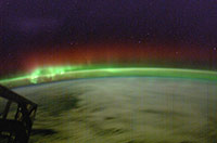
The aurorae are a striking phenomenon seen in polar regions, in which the thin air of the upper atmosphere glows and shimmers at night. They are also known as the northern and southern (or polar) lights. In this article, we explain how the aurorae are formed, and describe four activities, suitable for students aged 14-16, in which the aurorae and related phenomena can be simulated.
Perhaps unexpectedly, the ultimate cause of the aurorae lies not in Earth’s atmosphere, but in the Sun. The Sun – our star – releases its energy into space in two ways: as radiation, of which we see the visible part every day; and as solar wind, which is invisible, but which powers the aurorae when it interacts with the upper atmosphere. The solar wind is made up of charged particles – electrons and ions, primarily hydrogen ions (protons) – and has variable properties. Its velocity ranges from a few tens of kilometres per second to several thousand, and its density is in the range of a few (typically five) electrons and protons per cubic centimetre at Earth’s distance from the Sun.
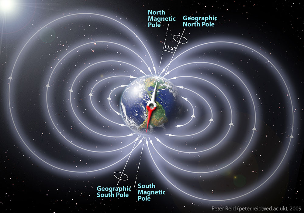
Being electrically charged, the solar wind is sensitive to magnetic fields. One consequence of this is that a large proportion of the solar wind particles that pass by our planet are trapped by Earth’s magnetic field (figure 1) and eventually directed toward one of Earth’s magnetic poles; these trapped particles form what is known as the Van Allen belt.
For the most part, the Van Allen belt lies far above Earth’s surface (about 45 000 km at the equator). At the poles, however, it enters the atmosphere: its charged particles collide with the atmosphere at an altitude of 80-500 km, where the air is very thin (with a pressure of less than a few tenths of a pascal).
How does this cause the aurorae? During the collisions, the atoms in the atmosphere become ionised (when one or more electrons are ejected) or excited (when the collision increases the energy level of an electron, but stops short of ejecting it), and therefore unstable.
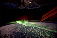
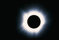
To return to their normal state, they must either undergo chemical reactions or release the energy they have just absorbed as light. When this process emits visible light, we call it an aurora. Seen from space, the northern and southern aurorae each form a ring known as an auroral oval, demarcating the region where the Van Allen belt plunges into Earth’s atmosphere (see image right).
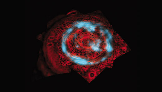
Although we are most familiar with the aurorae on Earth, they are not restricted to our own planet: astronomers have observed aurorae on other planets in the Solar System, particularly Jupiter and Saturn, and even Mars, above magnetic anomalies.
The Norwegian scientist Kristian Olav Birkeland (1867-1917) was the first to use a small magnetised sphere known as a terrella (‘small Earth’) to demonstrate the mechanisms of the aurorae. In a vacuum chamber, a cathode, representing the Sun, produces a stream of electrons (the solar wind, although in reality, electrons are only one component of the solar wind), while the terrella (the anode) is subjected to this wind and behaves like a planet or other body in the Solar System. The setup can be varied, as described below, to demonstrate a range of other physical phenomena.
The equipment can be easily built using materials commonly found in high schools, and takes about 10 hours to construct. The general setup is shown in figure 2; download details of the materials and constructionw1 from the Science in School website.
Care should be taken when working with high voltages. See also the general Science in School safety note.
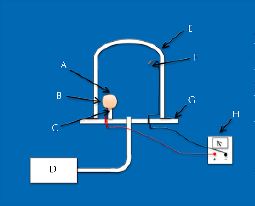
In this experiment, similar to Birkeland’s, we simulate the aurorae and the Van Allen belt. The equipment should be set up so that the electrode suspended from the top of the vacuum chamber is the cathode, representing the Sun and generating a stream of electrons (figure 2). The magnetic sphere is the anode, representing Earth, and its magnetic axis should be perpendicular to the stream of electrons.
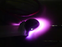
The electrons (‘solar wind’) are attracted to and envelop the sphere (‘Earth’, the anode). As they do this, they collide with gas atoms because the chamber is not a perfect vacuum, and we see this as a glow around the sphere. The electrons then move towards the poles of the sphere and loop under, following the magnetic field lines; we see this as a bright ring surrounding each pole (figure 3).
How does the simulation relate to reality? The generalised glow around the magnetic sphere represents the Van Allen belt, which in reality is only visible at the poles, where it enters Earth’s atmosphere. In our simulation, because there are small amounts of gas throughout the chamber, our ‘Van Allen belt’ visualises the entire magnetic field of ‘Earth’.
The bright rings around each pole in our simulation represent the auroral ovals. As in reality, they are caused by large numbers of electrons (remember that the magnetic field lines are closer together at the poles) striking gas atoms.
The colours in the simulation, however, differ from those most commonly seen in the northern and southern lights. The brightest colours in Earth’s aurorae (green and red) are caused by atomic oxygen, which is only present in the upper atmosphere. The colours in our simulation (purple, red, pink and white) are found in aurorae only at lower altitudes, where molecular oxygen and nitrogen are abundant. These colours are only visible a few times per decade when the solar wind enters the atmosphere at particularly high speeds.
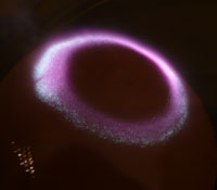
In the previous experiment, the sphere was the anode and represented Earth, while the other electrode represented a star (the Sun). In this experiment we swap the two, setting up the sphere as the cathode, to see the effect of the solar wind around a star. When we do this, we see a bright ring around the equator of the ‘star’ (figure 4).
What is happening? The electrons are circling the magnetic equator of the sphere under the influence of the Lorentz force (also known as Laplace force), which is created when a charged particle moves in a magnetic field. The force is perpendicular to both the particle’s direction of travel and the magnetic field, and therefore causes the particle to rotate around the magnetic field line. This creates a stellar ring current.
How does our simulation relate to reality? There is no ring current around the Sun because its magnetic field is not strong enough. It is possible, however, that ring currents may exist around other stars with stronger magnetic fields, but they cannot be observed with existing telescope technology because the stars themselves are much brighter than the ring current would be.
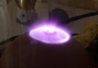
In this experiment too, we go beyond what has been observed in nature, creating an aurora on the Sun itself. Once again, we set up the sphere as the cathode, this time increasing the strength of the magnetic field using a stronger magnet and a sphere with a thinner wall (we used a Christmas tree bauble). When we do this, we see that the electrons are blown from the ‘Sun’ but a proportion of this ‘solar wind’ then falls back onto the Sun along its magnetic field lines, forming a dramatic circle of light at the pole closest to the anode, as seen in figure 5.
Does this reflect reality? Based on our understanding of the Sun and the solar wind, scientists predict that an aurora should exist around the Sun, but that we cannot observe it because the Sun is both too bright and too far away.
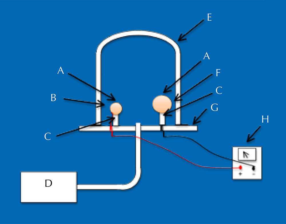
So far, our experiments have modelled either the Sun or Earth individually, representing the other with a simple electrode. However it is also possible to represent both bodies with spheres at the same time. In this activity, we dispense with the simple electrode and instead place two magnetic spheres in the vacuum chamber (figure 6), to demonstrate several phenomena related to the interaction between the Sun and Earth. For the Sun, we use the sphere from activity 3 (e.g. a Christmas tree bauble with a magnet inside it) as the cathode, and to represent Earth, a smaller spherical magnet as the anode.
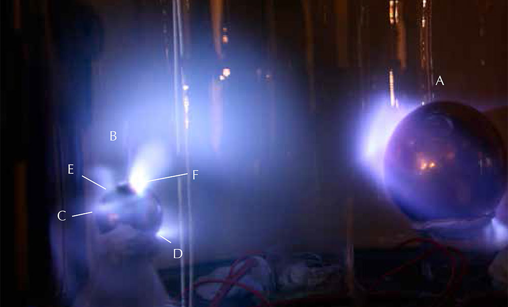
We see a glow all around the ‘Sun’ (figure 7A), similar to the generalised glow around ‘Earth’ in activity 1. This time, however, the glow represents the Sun’s corona. The solar corona is the expansion of the solar wind leaving the star, and is only visible from Earth during solar eclipses; the rest of the time it is outshone by the Sun’s surface. In reality, the formation of the solar corona depends not only on the solar wind but also on the temperature and the magnetic configuration of the Sun, so our ‘corona’ is more an analogy than a simulation.
The simulated solar wind travels from the Sun (figure 7A) through interplanetary space to Earth (B). There, as in activity 1, it causes a glowing envelope around the planet (the Van Allen belt), as well as bright rings around the poles (the auroral ovals). In figure 7, the northern auroral oval (C) is clearly visible and the southern one is hidden by part of our apparatus.
We can also see bright plumes of light on the auroral ovals (figure 7D, E and F). These plumes also exist in reality, and are known as the polar cusps. In our simulation, they are the result of the magnetic fields of the two spheres being directly linked: the electrons travel along the interconnecting magnetic field lines. In reality, the explanation is a little more complex: the Sun and Earth’s magnetic field lines are not directly connected to one another, but are linked through the interplanetary magnetic field, which is embedded in the solar wind.
In reality, unlike in our simulation, the auroral ovals are brighter than the polar cusps. This is because the acceleration of the charged particles that cause the auroral ovals increases as they enter Earth’s magnetic field, which increases the particles’ energy and velocity, brightening the aurora. In the simulation, the electrons travel at constant speed.
The article provides an introduction to the aurorae and the solar wind, and describes a very interesting way to simulate them at school. The teaching activity would be useful mainly for teaching physics or perhaps geography to students aged 16-19. Younger students would also enjoy the colourful and dramatic experiments even if they didn’t understand exactly what was being simulated.
The topic and the activity could be used as the basis of classroom discussions, because astrophysics is of huge interest to students. It would be an opportunity to link classic physics topics (e.g. electricity and ionisation) to modern physics (e.g. astrophysics and particle physics) or to have an interdisciplinary lesson linked to earth science (e.g. the Solar System).
Suitable comprehension questions include:
Gerd Vogt, Higher Secondary School for Environment and Economics, Yspertal, Austria