Supporting materials
Download
Download this article as a PDF


Pongprapan Pongsophon, Vantipa Roadrangka and Alison Campbell from Kasetsart University in Bangkok, Thailand, demonstrate how a difficult concept in evolution can be explained with equipment as simple as a box of buttons!
“The Hardy-Weinberg principle is the most difficult concept for me. I have not been clear about this topic since I started teaching it ten years ago. I know how to solve Hardy-Weinberg problems and can explain the procedures to students but…I really don’t see what we use it for and how it relates to evolution. To me, this topic is more mathematics than biology.”
Mrs Karnika, a secondary-school biology teacher in Bangkok
When, almost 150 years ago, Charles Darwin made public his theory of evolution by natural selection, the idea had one serious weakness. Like most biologists of his time, Darwin supposed that the characteristics of parents were ‘blended’ in the offspring. Over several generations this would, however, lead to a reduction in variation, giving natural selection little on which to operate. A chance encounter between a biologist and a mathematician on a cricket pitch some 50 years later played a crucial role in solving the problem.
The first steps were taken at the start of the 20th century, when Gregor Mendel’s work on inheritance in plants was rediscovered. It suggested that characteristics are discrete and do not blend. Mendel also observed that although a characteristic may seem to vanish in a particular generation, it is merely hidden by a ‘dominant’ characteristic – thus it can reappear, unchanged, in a subsequent generation.
Rather than bolstering Darwin’s theory, however, these discoveries were taken by many to be incompatible with natural selection. If the units of inheritance were discrete, how could the small, continuous variations observed by biologists be produced? And why, if Mendel was correct, didn’t the frequency of dominant characteristics increase in the population?
Unable to solve this latter problem, the British biologist Reginald Punnett asked G. Harold Hardy (with whom he played cricket) to help. Hardy, a pure mathematician, generally treated applied mathematics with contempt. In 1908 he wrote to the editor of the journal Science:
“I am reluctant to intrude in a discussion concerning matters of which I have no expert knowledge, and I should have expected the very simple point which I wish to make to have been familiar to biologists. However, some remarks … to which Mr. R. C. Punnett has called my attention, suggest that it may still be worth making….”
The ‘very simple point’ that Hardy went on to prove was that in a relatively large population where there is no migration, in which mating occurs at random and in the absence of selection or mutation, the frequency of genes will remain the same. Variation would be preserved over the generations.
‘Hardy’s principle’ contributed towards the reconciliation of Darwin’s natural selection with Mendelian genetics that developed gradually over the 1920s and 1930s to form our modern ideas about evolution.
In 1943 the principle became known as the Hardy-Weinberg principle (or the Hardy-Weinberg equilibrium or law) when it emerged that the same idea had been proposed independently in 1908 by a German physician, Wilhelm Weinberg.*
Today the science of population genetics, of which it is part, provides the most important theoretical basis for evolutionary biology and can be used to test almost all evolutionary ideas.
* It was later discovered that an American, William Castle, had suggested a similar idea in 1903.
Dean Madden, National Centre for Biotechnology Education, UK
The Hardy-Weinberg principle is one of the most difficult topics in evolution for many teachers and students (Mertens, 1992). They may feel threatened by mathematics and the quantitative aspects of population genetics, and may be unable to apply the principle to make sense of evolutionary phenomena. Many of them wonder about the relevance of the Hardy-Weinberg principle to understanding evolution. To help Mrs Karnika and other teachers who face the same difficulties, I would like to introduce the Counting Buttons activity. This is a simple demonstration of the Hardy-Weinberg equilibrium and how natural selection affects the allele frequency of a population. This activity is appropriate for high-school and university students studying evolution. The activity was originally developed by staff in the Department of Genetics at Kasetsart University in Thailand and later modified, as part of a PhD project, for use with high-school students.
Evolution is a change in allele frequency in a population over a period of time (Skelton, 1993; Strickberger, 1996). A population is a group of individuals of the same species in a given area whose members can interbreed and hence share a common group of genes known as a gene pool. Each gene pool comprises all alleles for all characteristics of all individuals. The allele frequency is the number of alleles of a given type as a proportion of the total number of alleles for that trait. In 1908, Hardy and Weinberg constructed a model of a population that was not evolving, and laid out the conditions in which such a population would exist (Abedon, 2005): a large population size with no migration, no mutation, no natural selection, and random mating. If we track allele frequencies in a population over a succession of generations and find that the frequencies of alleles deviate from the values expected from the Hardy-Weinberg equilibrium, then the population is evolving.
The Counting Buttons exercise simulates both a population in genetic equilibrium and a population undergoing natural selection. Natural selection acts on organisms’ phenotypes: physical traits, metabolism, physiology and behaviour, “and adapts a population to its environment by increasing or maintaining favorable genotypes in the gene pool” (Campbell & Reece, 2002). In a changing environment, natural selection favours any existing genotypes that have already adapted to the new conditions.
Note to teachers: Teachers should review students’ understanding of Mendelian genetics, especially monohybrid crosses, before running this exercise. This is an activity for groups of four to five students, and should take three hours.
After completing this activity, students will have simulated a population at genetic equilibrium and examined the effect of natural selection on the allele frequency of a population over five generations.
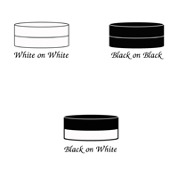
Each button represents one diploid individual in a population. Each side of the button represents an allele: black on black is an individual with genotype RR, black on white is Rr, and white on white is rr.
Each pair of buttons will produce four offspring; the genotypes of the offspring are determined according to Mendel’s first law.
Experiment I: a population at equilibrium
Experiment II: an evolving population
Suppose the individuals with genotype rr die out before they reproduce. You will need to eliminate white/white buttons from each generation after the first.
Note: The students might find that, in some rounds, there is a single unpaired button left in the box after selecting pairs of buttons. This remaining button must be removed from the population because it does not have a chance to mate with other individuals.
The complete tables can be downloaded from the Science in School websitew1
| No. | Genotypes of parents | Genotypes of offspring | ||||
|---|---|---|---|---|---|---|
| PR | Rr | rr | ||||
| 1 | → | |||||
| 2 | → | |||||
| 3 | → | |||||
| 4 | → | |||||
| 5 | → | |||||
| Generations | Number of each genotype | Frequency of allele R | Frequency of allele r | ||
|---|---|---|---|---|---|
| RR | Rr | rr | |||
| 0 | 16 | 32 | 16 | 0.5 | 0.5 |
| 1 | |||||
| 2 | |||||
| 3 | |||||
| 4 | |||||
| 5 | |||||
| Generations | Number of each genotype | Frequency of allele R | |||
|---|---|---|---|---|---|
| RR | Rr | Frequency of allele rrr | |||
| 0 | 16 | 32 | 16 | 0.5 | 0.5 |
| 1 | |||||
| 2 | |||||
| 3 | |||||
| 4 | |||||
| 5 | |||||
When there is no selection pressure, the frequency of the two alleles fluctuates slightly (Table 5). When there is a selective pressure against the homozygous recessive genotype (that is, if rr individuals die before they reproduce), the frequency of the r allele in the population declines over time (Table 6).
| NO. | Genotypes of offspring | |||||
|---|---|---|---|---|---|---|
| RR | Rr | rr | ||||
| 1 | RR | Rr | → | 2 | 2 | 0 |
| 2 | → | |||||
| 3 | → | |||||
| 4 | → | |||||
| 5 | → | |||||
| Generation | Number of each genotype | requency of allele R | Frequency of allele r | ||
|---|---|---|---|---|---|
| RR | Rr | rr | |||
| 0 | 16 | 32 | 16 | 0.5 | 0.5 |
| 1 | D1 = 17 | H1 = 34 | R1 = 13 | 0.53 | 0.47 |
| 2 | D2 = 14 | H2 = 35 | R2 = 15 | 0.49 | 0.51 |
| 3 | D3 = 16 | H3 = 32 | R3 = 16 | 0.50 | 0.50 |
| 4 | D4 = 15 | H4 = 31 | R4 = 18 | 0.48 | 0.52 |
| 5 | D5 = 16 | H5 = 33 | R5 = 15 | 0.50 | 0.50 |
| Generation | Number of each genotype | Frequency of allele R | Frequency of allele r | ||
|---|---|---|---|---|---|
| RR | Rr | rr | |||
| 0 | 16 | 32 | 16 | 0.5 | 0.5 |
| 1 | D1 = 21 | H1 = 29 | R1 = 14 | 0.55 | 0.45 |
| 2 | D2 = 30 | H2 = 24 | R2 = 10 | 0.65 | 0.35 |
| 3 | D3 = 36 | H3 = 21 | R3 = 17 | 0.72 | 0.28 |
| 4 | D4 = 41 | H4 = 17 | R4 = 6 | 0.77 | 0.23 |
| 5 | D5 = 48 | H5 = 12 | R5 = 4 | 0.84 | 0.16 |
D = dominant
H = heterozygous
R = recessive
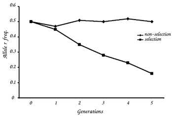
Compare the graphs of allele frequency from the stable and the evolving population. Do they differ?
How does natural selection affect allele frequencies of a population over time?
Will a dominant allele of a trait always have the highest frequency in a population and a recessive allele always have the lowest frequency? Explain your answer.
Teachers should be aware that students may misinterpret the graphs, focusing only on two or three points and not noticing that there are fluctuations from generation to generation. The teacher should also emphasise that in a natural population it usually takes more than five generations before we can detect any change in allele frequency. Evolution takes time.
After conducting the second experiment, some students might conclude that natural selection always increases the frequency of a dominant allele and decreases the frequency of a recessive allele in a population. However, not all selections would result in a progressive decrease in a recessive allele. The allele – dominant or recessive – that is selected out is determined by the environmental conditions at the time. In order to avoid this misunderstanding, it is advisable for the teacher to ask the students to consider examples in which the recessive allele is common, or the dominant allele is rare: type O blood is a recessive trait but the majority of people in some populations have this blood type; Huntington’s disease is a dominant trait but only 4-10 individuals in 100 000 have it. More examples of other kinds of natural selection are described in O’Neil (2006).

Counting Buttons is a simple and concrete way to demonstrate the Hardy-Weinberg principle. By engaging in this activity, students will gain insight into a population at equilibrium and into natural selection as a force for biological adaptation. Students will have to apply Mendelian law and mathematical skills to make sense of the data and interpret the results. Counting Buttons is an example of how to teach biology in an integrated fashion and to use mathematics to make sense of complex biological phenomena.
“Counting Buttons helped me make sense of the Hardy-Weinberg principle. Now, I can explain to students what the principle is used for and how to link it to other topics of evolution meaningfully. I feel more confident and enjoy teaching this topic. Obviously, the students paid more attention to the lesson. They were very happy to work hands-on and collaboratively in this lab exercise.”
Mrs Karnika, after running Counting Buttons
At any level, the Hardy-Weinberg principle is a difficult concept to grasp. It is virtually impossible to see how it acts and how selection may affect the frequency of alleles. This ingenious idea for active learning of a seemingly abstract concept simulates how the Hardy-Weinberg principle applies to both a stable and an evolving population. Buttons representing homozygous dominant and recessive, and heterozygous, genotypes are used to review the understanding of Mendelian genetics and then to investigate how allele frequency changes in stable and evolving populations.
Three hours for the whole activity is a reasonable estimate. The activity would be ideal as two separate lessons: one for a stable population and one for an evolving population. This will prevent the students from becoming bored with pulling buttons out of bags or confused by the different mathematics required to model each population. The mathematics for the evolving population requires some concentration to understand and may take students a while to calculate.
The questions for discussion should provoke some good exchange of ideas. The points made about allele selection would raise awareness of some dominant and recessive genetic diseases and could be used for further research, perhaps linking them into genetic engineering and genetic diagnosis and, if time permits, debates on the ethics of selection.
Shelley Goodman, UK
Download this article as a PDF