


Grow your own statistical data Teach article
Would your students prefer to grow edible crops or wrangle with statistics? Here’s a way to combine these activities in a real-world application of statistical analysis.
Most biology students prefer to avoid mathematics, which is often one of the reasons they chose biology. So in the senior classes (age 16–18), when statistical tests are mentioned, the whole class groans – and quite often the teacher as well.

always the aspect that most
interests students
Sean/Flickr CC BY-ND 2.0
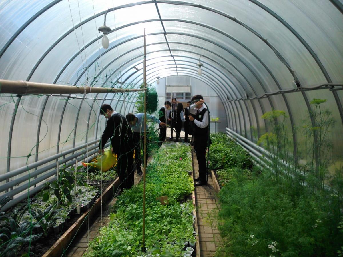
In 2018, we were carrying out project work in our school in Kazakhstan, growing plants in the school greenhouse with some of the junior classes. At the same time, the older biology students were studying the t-test, which is a standard way to evaluate an experimental hypothesis. Introducing maths into biology lessons is not easy, so it occurred to us that it might be more exciting to use the data collected in the plant-growing project for some real-life data analysis.
The t-test is one of several standard statistical tests used to find out whether there is a ‘statistically significant’ difference between two related sets of data – that is, whether any such difference could have occurred just by chance. Growing plants under two different conditions – in normal and in enriched soil – could provide a hypothesis to test and two good data sets for statistical analysis.
The idea was a success: we found that using data from an actual experiment in school made the statistical analysis seem more real, and students could see how the t-test enables us to draw conclusions in everyday life, rather being a purely paper-based exercise.
In this article, we describe both stages of this activity: the greenhouse project and the subsequent statistical analysis using the t-test. The greenhouse activity is suitable for students aged 14–16 and takes around eight hours of class time, plus 10–12 weeks for the plants to grow. The t-test activity is suitable for students aged 16–18 and takes around four hours.
For some definitions of statistical terms, please see the text box (or use standard sources).
Joanne Brown
Stage 1: Growing plants in a greenhouse
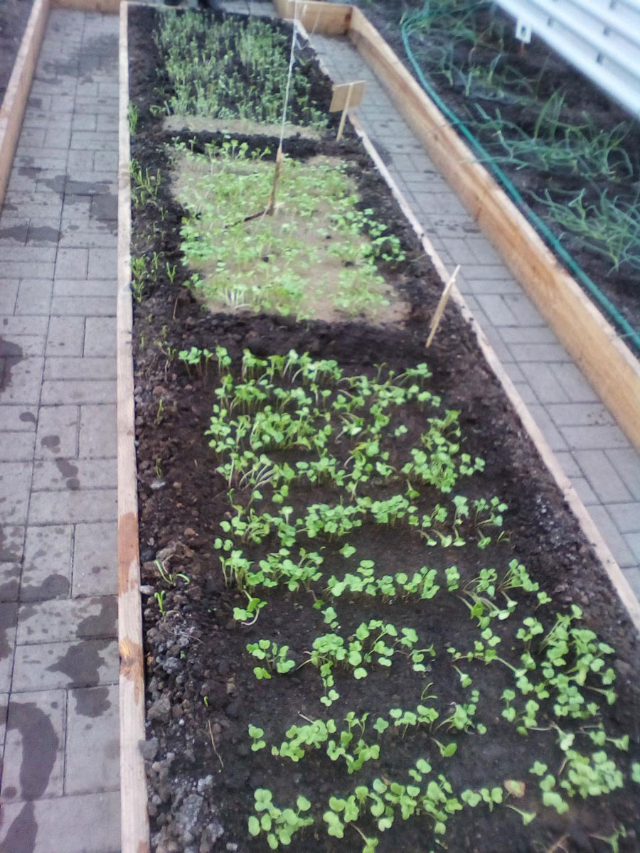
(top) are lighter in colour
than the normal plots
(bottom).
Joanne Brown
Most students like to see plants grow, so the horticulture experiment is a worthwhile activity in itself. Kazakhstan has a continental climate, with very hot summers and extremely cold winters, so to grow plants in the spring we used a heated greenhouse. Of course, the plants can also be grown outdoors if the season and climate are suitable.
Most importantly, choose a clear hypothesis and two clearly distinct growing conditions to test the hypothesis. We chose the following:
Aim of experiment: To determine if enriching the soil with nutrients increases the growth of radish leaves.
Hypothesis: Radish plants grown in nutrient-enriched soil will have bigger leaves.
For the enriched soil, we added farmyard manure containing potassium (1.3%), nitrogen (0.1%) and magnesium (0.6%).
Materials
- Radish seeds (approximately 160 in total, or 10 seeds per plot)
- Area of normal soil for planting, at least 16 m2
- Farmyard manure (4 kg in total, or 500 g per plot)
- Spades
- Watering can
- Tape measure
- Ruler
- Calculator
Procedure
The students can carry out the steps needed to grow the plants.
Safety note:
Always wash your hands after handling soil or manure.
- To prepare the soil, use the spade to dig the soil and turn it over until it is quite finely divided.
- Measure out 16 plots of 1 m2 each using the tape measure: eight for the enriched soil and eight for the normal soil. Mark out the plots using string, then label each plot with the plot number.
- Add 500 g farmyard manure to each of the eight enriched plots. Use the spades to mix this in well with the soil.
- Plant ten radish seeds per plot, approximately 100 mm apart and 10 mm deep.
- Water the plants every day, or as needed. Observe the growth of the plants over about seven weeks, from germination to seedlings and then to fully developed plants.
- On one day each week (e.g. Friday) throughout the growing period, use a ruler to measure the length of the biggest leaf from each plant in all 16 plots. Record these measurements carefully.
At the end of the growing period, calculate the mean (average) length of these leaves for each plot over the whole growing period. This is calculated by adding together all the measurements for that plot, and then dividing the result by the number of measurements.
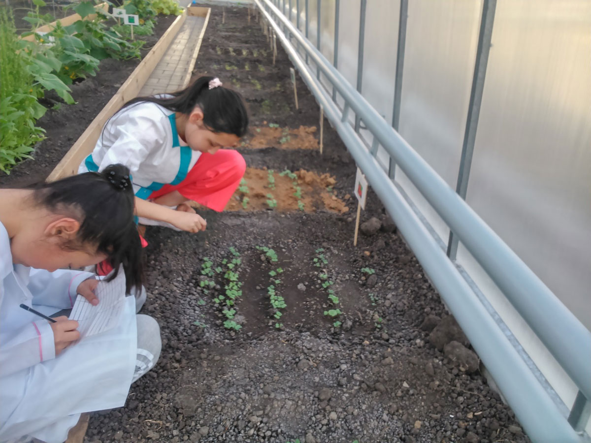
Joanne Brown
Results and conclusions
In our experiment, 67 radish plants germinated in the plots with the enriched soil and 99 radish plants germinated in the normal soil (the numbers differed because it was difficult to count all the seeds accurately, plus some seeds didn’t germinate).
The table below shows the mean lengths of the biggest leaves for plants in each plot over the growing period, and the overall mean in each condition.
| Enriched soil: Plot numbers | Mean length of biggest leaf from plants in each plot (mm) | Normal soil: Plot numbers | Mean length of longest leaf from plants in each plot (mm) | |
|---|---|---|---|---|
| 1 | 39 | 9 | 38 | |
| 2 | 45 | 10 | 41 | |
| 3 | 41 | 11 | 43 | |
| 4 | 46 | 12 | 39 | |
| 5 | 45 | 13 | 37 | |
| 6 | 48 | 14 | 38 | |
| 7 | 39 | 15 | 41 | |
| 8 | 44 | 16 | 36 | |
| Overall mean (enriched soil) | 43.38 | Overall mean (normal soil) | 39.13 |
As these results show, the leaves were indeed bigger on average in the plots with the added nutrients, in line with our hypothesis.
For a junior class, it’s adequate to conclude that this result agrees with the hypothesis. However, at a more senior level (and in real science), we would need to show that this result is unlikely to have occurred by chance – in other words, that it is statistically significant. This is the aim of the next stage of the activity.
Stage 2: Using the t-test
The results from the horticulture experiment can be used as ‘real’ data for advanced students to analyse using the t-test.
The t-test is used to determine if there is a statistically significant (i.e. non-chance) difference between the means of two related sets of data, and thus between results from two different experimental conditions. In this case, the students investigate whether enriching the soil has made a statistically significant difference in the size of radish leaves, compared to normal soil, or whether the difference in mean leaf size could have occurred by chance.
Procedure
To use the t-test, we need the two data sets from the plant-growing experiment (normal and enriched soil). We then follow a standard mathematical process to analyse the data and find out whether it supports our chosen hypothesis.
Step 1: Decide on the null hypothesis, H0
To find out using the t-test if a hypothesis is supported by data, we first need to decide on a ‘null hypothesis’. In general, this is the hypothesis that the different conditions made no difference to the results. So if the data analysis shows we can reject this hypothesis, then we can conclude that the different conditions did make a difference to the results.
Here, the null hypothesis, H0, is:
There will be no significant difference in the average size of radish leaves growing in enriched soil and those growing in normal soil.
Step 2: Calculate the standard deviation in each condition
Next, we calculate the standard deviation (SD) for each of the two data sets.
Standard deviation (SD) =
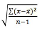
Where:
x = mean measurement for each soil plot (see table 1)
x̅ = average of the means from all the measurements in one condition (enriched soil, normal soil); see table 1
n = number of measurements in each condition (8 in this case)
For example, in plot 1:
x = 39
x̅ = 43.38
So (x – x̅)2 = (39 – 43.38)2 = 19.18
The completed results are shown in table 2.
| Plot number | Enriched soil, size of leaves (mm) | (x – x̅)2
x̅ = 43.38 |
Plot number | Normal soil, size of leaves (mm) | (x – x̅)2
x̅ = 39.13 |
|
|---|---|---|---|---|---|---|
| 1 | 39 | 19.18 | 9 | 38 | 1.28 | |
| 2 | 45 | 2.62 | 10 | 41 | 3.50 | |
| 3 | 41 | 5.66 | 11 | 43 | 14.98 | |
| 4 | 46 | 6.86 | 12 | 39 | 0.02 | |
| 5 | 45 | 2.62 | 13 | 37 | 4.53 | |
| 6 | 48 | 21.34 | 14 | 38 | 1.28 | |
| 7 | 39 | 19.18 | 15 | 41 | 3.50 | |
| 8 | 44 | 0.38 | 16 | 36 | 9.80 | |
| Total | 77.84 | Total | 38.89 |
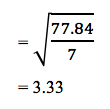
So the standard deviation for enriched soil (SD1):
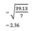
The standard deviation for normal soil (SD2):
Step 3: Calculate the overall t-value
We can now determine the t-value using the equation below:
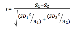
Where:
x̅1= mean of the results in the first condition (enriched soil)
x̅2 = mean of the results in the second condition (normal soil)
n1 = number of measurements in first condition
n2 = number of measurements in second condition
So:
x̅1 – x̅2 = 43.48 – 39.13
= 4.25
SD12= 3.332 = 11.09
SD22 = 2.362 = 5.57
n1 = n2 = 8
11.09/8 = 1.39
5.57/8 = 0.70
So
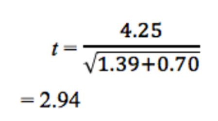
In the next steps, we will use this t-value to find out if the data supports the null hypothesis, or if we should reject it.
Step 4: Find the ‘degrees of freedom’
The ‘degrees of freedom’ in a statistical calculation is a mathematical concept that represents how many values involved in a calculation have the freedom to vary. The lower the degrees of freedom, the higher the t-value needs to be for statistical significance.
We find the degrees of freedom by:
- adding the sample sizes (number of measurements) in both conditions, then
- subtracting 2.
So here, the value for the degrees of freedom is 16 – 2 = 14
Step 5: Check the critical value and compare this to the t-value obtained
Using the value calculated for the degrees of freedom, we can read off the ‘critical value’ from the standard figures shown in the table below.
If the t-value is more than the critical value, there is a statistically significant difference between the results in the two conditions. This means there is a probability of not more than 5% (at p ≤ 0.05) that the difference occurred by chance.
| Degrees of freedom | Critical value for significance (at p ≤ 0.05) |
|---|---|
| 1 | 12.71 |
| 2 | 4.30 |
| 3 | 3.18 |
| 4 | 2.78 |
| 5 | 2.57 |
| 6 | 2.45 |
| 7 | 2.36 |
| 8 | 2.31 |
| 9 | 2.26 |
| 10 | 2.23 |
| 11 | 2.20 |
| 12 | 2.18 |
| 13 | 2.16 |
| 14 | 2.14 |
| 15 | 2.13 |
Here, t = 2.94 and the critical value is 2.14, so the t-value exceeds the critical value. This means we can reject the null hypothesis, as it is overwhelmingly likely that the difference in the results did not occur by chance.
Conclusion and discussion
In this investigation, the value of t was more than the critical value at the relevant degree of freedom, so we therefore reject the null hypothesis. Thus, we can conclude that there is a statistically significant difference in the size of the leaves growing in the enriched soil compared to the normal soil.
As well as discussing the statistical conclusion, students might like to critique the overall experiment and suggest any factors that could have affected the results. Can they propose any improvements?
Additionally, are there other data sets that might be interesting to collect and analyse using the t-test?
What did we learn from the project?
For the junior students, who like to see plants grow, getting out of the classroom into the greenhouse during the lesson does encourage them. In the next academic year, we will grow plants that appeal more to the students’ tastes, such as tomatoes and sugar snap peas, rather than radishes.
For the senior students, we found that these activities helped them to develop their statistics skills, as well as to gain a better understanding of hypothesis testing, which is an essential part of any practical work in biology. Our students now understand what ‘statistical significance’ actually means!
Definitions
| p-value | The p-value is a number between 0 and 1 that determines the statistical significance of your results. A small p-value (usually ≤ 0.05) indicates strong evidence against the null hypothesis, so you reject the null hypothesis. |
| Degrees of freedom | The degrees of freedom in a statistical calculation represent how many values involved in a calculation have the freedom to vary. This is an important factor in finding out whether results are statistically significant. |
| Standard deviation | The standard deviation is a measure used to quantify the amount of variation in a set of data values. A low standard deviation indicates that the data points are close to the mean of the data set, while a high standard deviation indicates that the data points are spread over a wider range of values. |
| Null hypothesis, Ho | A null hypothesis expresses the idea that any difference between sets of data is due to chance. |
| Statistical significance | In biology, a result is statistically significant if the probability of the null hypothesis being correct is 5% or less (p ≤ 0.05). So a statistically significant result means we are 95% sure that Ho is not correct. |
Resources
- Find out more about the t-test and its applications in biology on the Biology for Life website.
- Download this resource from the school exam board OCR on the different statistical tests and how to decide which one to select.
- Understand more about degrees of freedom from the Statistics by Jim website.
Review
This article shows how junior and senior biology classes can cooperate to test a hypothesis through experimentation. The junior classes do an experiment growing plants outdoors, which generates data that is used by the senior classes to analyse with statistical methods.
While the activity of growing plants and measuring their growth is not especially novel, coupling this with a statistics exercise provides a useful way to teach data interpretation in biology – and the importance of correct statistical evaluation in science.
The activities also provide an opportunity to increase cooperation between classes. The senior students could consider how to improve the experiment to obtain better data – for example, which variable in the plant growth experiment would be most suitable to measure, and why – and then share their ideas with the junior students.
Monica Menesini, science teacher, Italy